1 Introduction
Consider a complete market model framework with the unique equivalent local martingale measure ${Q^{e}}$. In the spirit of Reichlin [19], we consider a utility function U on ${\mathbb{R}_{+}}$ which is nondecreasing upper-semicontinuous and satisfying a mild growth condition. Schied and Wu [21] impose the below assumptions on the set of probability measures $\mathcal{Q}$ on $(\Omega ,\mathcal{F})$; note that $\mathcal{Q}$ is not the set of all measures on the measurable space $(\Omega ,\mathcal{F})$, but just a subset satisfying these assumptions.
Assumption 1.
Also, to Assumption 1 we add
where ${\mathcal{Q}_{e}}$ denotes the set of measures in $\mathcal{Q}$ that are equivalent to $\mathbb{P}$.
In this paper we study the minimax identity for the robust nonconcave utility functional in a complete market model, i.e.
\[ u(x):=\underset{X\in \mathcal{X}(x)}{\sup }\underset{Q\in \mathcal{Q}}{\inf }{E_{Q}}[U(X)]=\underset{Q\in \mathcal{Q}}{\inf }\underset{X\in \mathcal{X}(x)}{\sup }{E_{Q}}[U(X)],\]
while considering two possibilities for the set $\mathcal{X}(x)$ of admissible final endowments:One of the key tasks of financial mathematics is proving the existence as well as the construction of optimal investment strategies, in other words, finding the utility-maximizing investment strategies. Mostly, this problem was studied under the assumption that the probability distribution of the value process is known.
However, in reality, along with the exact probabilities unknown, there are abundant aspects that can be considered in mentioned maximization problems such as the completeness of the market, the set of prior probability measures, the assumptions on investor’s utility function, the modeling of payoff and so on. That is why instead of a single measure it is sound to consider the set of probability measures with natural assumptions on it. Thus, the standard utility maximization problem becomes the robust utility maximization problem
where one maximizes the expected utility under the infimum over the whole set of probability measures, for details see Gilboa and Schmeidler [9, 10, 22], Yaari [25], Föllmer and Schied [8, Section 2.5].
In the case of a standard utility maximization problem it is possible to construct the optimal investment strategy given a strictly concave utility function, see Föllmer and Schied [8, Section 2.5], and for the general utility functions, see Bahchedjioglou and Shevchenko [4]. Both references considered standard budget constraints as well as an additional upper bound on the final endowments. For a detailed survey of this problem in a general model setup in both complete and incomplete market models but with risk-averse agent, see Biagini [6].
In this paper, we consider the robust maximization problem with the general nonconcave utility function, with and without budget constraints likewise. In the previous literature different approaches were used for robust portfolio optimization such as reducing the robust case to the standard one through proving the existence of the “worst-case scenario measure” or “the least favorable measure”, e.g., [17, 20], a stochastic control approach, see [11], an approach using BSDEs, see [7] and references therein.
Besides, for solving the optimal investment problems one can make use of the following interim finding such as minimax identity and duality theory. Using the minimax identity for concave functions, see [1, section 6], Schied and Wu [21] showed the existence of an optimal probability measure $\widehat{Q}$ in the sense that
\[ \underset{X\in \mathcal{X}(x)}{\sup }\underset{Q\in \mathcal{Q}}{\inf }{\mathrm{E}_{Q}}[U({X_{T}})]=\underset{X\in \mathcal{X}(x)}{\sup }{\mathrm{E}_{\widehat{Q}}}[U({X_{T}})],\]
which, together with the results of the Kramkov and Schachermayer [13, 14], was the base for proving the existence of the optimal investment strategy. They used a general incomplete market model with rather natural assumptions on the set of probability measures. Backhoff Veraguas and Fontbona [3] extended these results by implementing the assumption on the densities of the uncertainty set instead of the usual compactness assumption. Moreover, they have done this without relying on the existence of the worst-case measure or on any assumption implying this.Neufeld and Šikić [15, 16] studied a robust stochastic optimization problem in the quasi-sure setting in discrete time. Their paper [15] deals with the study of general concave utility functions, showing the existence of the maximizer in different market models under the linearity-type condition, which is caused by the no-arbitrage condition. In [16], they consider the nonconcave utility maximization problem and outline the conditions of maximizer’s existence.
For more results concerning the robust utility maximization problem we refer to Bartl, Kupper and Neufeld [5] and references therein.
The majority of articles on utility maximization assume that the investor’s utility function is strictly concave, strictly increasing, continuously differentiable, and satisfies the Inada conditions. While the assumption of monotonicity is natural, since an agent prefers more wealth to less, other assumptions can be omitted or relaxed. There is a wide class of models in which the maximization of the nonconcave and not necessarily continuously differentiable utility function has been studied by reducing the problem to the concave case. One of the most important works was done by Reichlin [18, 19]. He considered the general framework of nonconcave utility functions for both complete and incomplete market models. By applying the concavification technique he established valuable relations between the maximization problems for a nonconcave utility function U and its concavification ${U_{c}}$ thereby reducing the task to the concave problem. Moreover, Reichlin proved the existence of the maximizer under certain assumptions and established its properties.
While considering two cases of admissible final endowments – the standard budget constraint and additional upper bound (which has not been considered before in such model setup) – we extend Reichlin’s results by proving new connections in the form of equalities and inequalities of the robust utility maximization functionals of initial nonconcave utility functions and its concavification. Furthermore, we proceed in proving the minimax identity for general nonconcave utility functions. The crucial step for obtaining the mentioned results with implementing an additional upper bound is the use of the regular conditional distribution which sheds new light on the possible approaches for solving the optimization problem.
The paper is organized as follows. In Section 2 we study the minimax identity for a nonconcave utility function in the complete market model. We do not prove nor refute the minimax identity, however, we show useful equalities and inequalities to relate the robust utility functional of initial utility function and its concavification. Section 3 is devoted to the study of the minimax identity under the implementation of budget constraints. The results of Section 3 are similar to the corresponding results of Section 2, however, some of proves differ significantly.
Throughout the paper the measurability of real-valued functions is understood in the Borel sense.
2 Minimax identity for nonconcave utility functions in complete market model
This problem is already solved in [12], but, since we want to expand this problem by considering budget constraints, we present the main part of the mentioned paper omitting the proofs.
2.1 Formulation of the problem
To formulate the goal of this paper first let us remind some notations. For any initial capital $x>0$, let $\mathcal{X}(x)$ be the set of all possible random endowments corresponding to x, i.e. all random variables X such that $X\ge 0$, ${\mathrm{E}_{{Q^{e}}}}[X]\le x$.
Moreover, we consider a utility function U which is nondecreasing, upper-semicontinuous, defined on a domain $(0,\infty )$ and satisfying the mild growth condition:
It follows from [2, Proposition 3.1] that $U(x)$ has a nondecreasing and continuous concave envelope ${U_{c}}(x)$, or the smallest concave function such that ${U_{c}}(x)\ge U(x)$ for all $x\in \mathbb{R}$; we will call it a concavification of U.
This section aims to prove some equalities and inequalities related to the minimax identity for the robust nonconcave utility functionals:
We will assume that the probability space $(\Omega ,\mathcal{F},\mathbb{P})$ is atomless. Introduce the notation:
\[\begin{array}{l}\displaystyle {u^{c}}(x):=\underset{X\in \mathcal{X}(x)}{\sup }\underset{Q\in \mathcal{Q}}{\inf }{E_{Q}}[{U_{c}}(X)];\\ {} \displaystyle {u_{Q}}(x):=\underset{X\in \mathcal{X}(x)}{\sup }{E_{Q}}[U(X)];\\ {} \displaystyle {u_{Q}^{c}}(x):=\underset{X\in \mathcal{X}(x)}{\sup }{E_{Q}}[{U_{c}}(X)].\end{array}\]
Also, we need the finiteness of value functions, which we can write as follows.
Note that finiteness of ${u_{Q}^{c}}(x)$ implies finiteness of ${u_{Q}}(x)$, since ${u_{Q}}(x)\le {u_{Q}^{c}}(x)$.
Theorem 1.
Suppose that Assumptions 1, 2, 3 hold and that the probability space $(\Omega ,\mathcal{F},\mathbb{P})$ is atomless.
Then the following holds: 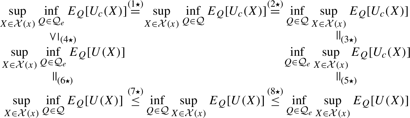
The proof of this theorem will be divided into several parts.
2.2 Minimax identity for the concavified objective function ${U_{c}}(x)$
Now we are going to show that the minimax identity holds for ${U_{c}}(x)$.
There is a lot of literature with proofs of the minimax identity for robust utility functionals, the most general case was considered in [21]. However, there the authors assume that the utility function is strictly increasing, strictly concave, and satisfies the Inada conditions both at point 0 and at ∞.
The function ${U_{c}}(\cdot )$ which we are considering is no longer strictly concave and does not satisfy the Inada conditions at 0, hence we cannot use all the previous results without changes.
The next lemma is almost the same as [21, Lemma 3.4].
Lemma 1.
Then we have
\[\begin{array}{l}\displaystyle {u^{c}}(x)=\underset{X\in \mathcal{X}(x)}{\sup }\underset{Q\in \mathcal{Q}}{\inf }{E_{Q}}[{U_{c}}(X)]=\underset{Q\in \mathcal{Q}}{\inf }\underset{X\in \mathcal{X}(x)}{\sup }{E_{Q}}[{U_{c}}(X)]\\ {} \displaystyle =\underset{X\in \mathcal{X}(x)}{\sup }\underset{Q\in {\mathcal{Q}_{e}}}{\inf }{E_{Q}}[{U_{c}}(X)]=\underset{Q\in {\mathcal{Q}_{e}}}{\inf }\underset{X\in \mathcal{X}(x)}{\sup }{E_{Q}}[{U_{c}}(X)].\end{array}\]
2.3 Minimax identity for the objective function $U(x)$
In this section, we want to prove lemmas which will help us to complete the proof of Theorem 1.
Remark.
Note that the main argument in the proof of minimax identity for the robust utility maximization problem is the lop sided minimax theorem by Aubin and Ekeland, see [1, Chapter 6, p. 295], which holds if the functional $X\to \mathbb{E}[ZU(X)]$ is concave. Since we consider the nonconcave utility function U, we cannot prove the minimax identity in this case similarly. A more general case of the minimax identity was proved by Maurice Sion, see [24]. However, to use Sion’s minimax theorem we still need functional $X\to \mathbb{E}[ZU(X)]$ to be quasi-concave, which is not true, in the general case, even for the indicator functions multiplied by the constants.
The proof of equality $(5\mathrm{\star })$ is based on [19, Theorem 5.1].
□
Proof of Theorem 1.
-
• $(4\mathrm{\star })$ follows from the fact that ${U_{c}}\ge U$;
-
• To obtain $(6\mathrm{\star })$ we need to take the $\underset{g\in C(x)}{\sup }$ of the both sides in equality (2);
-
• Since ${\mathcal{Q}_{e}}\subseteq \mathcal{Q}$, inequality $(8\mathrm{\star })$ is clear.
3 Minimax identity for constrained case of random endowments
3.1 Formulation of the problem
This section is in general similar to Section 2, however, similarly to [8, Chapter 3] we consider a modified constrained counterpart.
Specifically, we assume that there is an upper bound on the endowment, given by a random variable $W:\Omega \to (0,+\infty )$. The set of admissible payoffs is then given by
\[ {\mathcal{X}^{W}}:=\{X\in {L^{0}}(\mathbb{P})\mid 0\le X\le W\hspace{2.5pt}\mathbb{P}\text{-a.s.}\}.\]
As it was pointed out in [8, Chapter 3], such formulation arises in various applications. For instance, we can consider an agent who aims at reaching a certain random final wealth W; this may be the future price of certain asset or the claim that agent will have to pay. In this situation, additional utility for any amount above W is zero, while the agent still applies her utility function for endowments below W. Since we assume completeness, there is no reason to consider endowments X, which exceed W with positive probability, as they can safely be replaced by $X\wedge W$.We keep all of the assumptions from Section 2 on the set of all probability measures $\mathcal{Q}$ and the utility function U intact. For technical reasons we will also assume that $(\Omega ,\mathcal{F})$ is a standard Borel space, which in particular implies the existence of a regular conditional distribution given W. We will require that this conditional distribution is atomless, in other words, that the constraint W leaves a sufficient amount of randomness.
Assumption 4.
-
1. $(\Omega ,\mathcal{F})$ is a standard Borel space.
-
2. There exists a regular conditional distribution given W, which is atomless, i.e. there exists a function $P:\mathcal{F}\times (0,\infty )\to [0,\infty )$ such that for all $v>0$, $P(\cdot ,v)$ is an atomless probability measure, and for all $A\in \mathcal{F}$, $P(A,\cdot )$ is a measurable function satisfying $P(A,W)=\mathbb{P}(A\mid W)$ a.s.
Remark 2.
A simple sufficient condition for $(\Omega ,\mathcal{F})$ to be Borel is that $\mathcal{F}$ is generated by a collection of real-valued random variables, which is sufficient for the majority of applications. Since we assume market completeness, this assumptions is automatically fulfilled as long as one does not consider completion of $\mathcal{F}$.
The second assumption is verified if, for example, on $(\Omega ,\mathcal{F},\mathbb{P})$ there is a random variable which is independent of W and has continuous distribution, so it does not seem to be too restrictive. We also stress that it does not contradict the market completeness; the simplest example is a market with two independent continuously distributed assets ${S^{1}},{S^{2}}$ and $W=f({S^{1}})$.
Note that the function ${U^{k}}$ and its concavification ${U_{c}^{k}}$ satisfy all of the assumptions on the utility function U and its concavification ${U_{c}}$. Moreover, ${U_{c}^{k}}(x)={U^{k}}(x)$, for all $x\ge k$.
Our goal is to prove some equalities and inequalities related to the minimax identity for the robust nonconcave utility functionals
\[ \underset{X\in {\mathcal{X}_{x}^{W}}}{\sup }\underset{Q\in \mathcal{Q}}{\inf }{E_{Q}}[{U^{W(\omega )}}(X)]=\underset{Q\in \mathcal{Q}}{\inf }\underset{X\in {\mathcal{X}_{x}^{W}}}{\sup }{E_{Q}}[{U^{W(\omega )}}(X)]\]
with the budget set ${\mathcal{X}_{x}^{W}}$ defined by
where $x>0$ is the initial wealth and ${Q^{e}}$ is the unique equivalent local martingale measure.Introduce the following notation:
\[\begin{array}{l}\displaystyle {u_{c}^{W}}(x):=\underset{X\in {\mathcal{X}_{x}^{W}}}{\sup }\underset{Q\in \mathcal{Q}}{\inf }{E_{Q}}[{U_{c}^{W(\omega )}}(X)];\\ {} \displaystyle {u_{Q}^{W}}(x):=\underset{X\in {\mathcal{X}_{x}^{W}}}{\sup }{E_{Q}}[{U^{W(\omega )}}(X)];\\ {} \displaystyle {u_{c,Q}^{W}}(x):=\underset{X\in {\mathcal{X}_{x}^{W}}}{\sup }{E_{Q}}[{U_{c}^{W(\omega )}}(X)].\end{array}\]
It is natural to consider only the case where
as otherwise, thanks to the monotonicity of U, the optimization problem has a trivial solution ${X^{\ast }}=W$.
The formulation of the next theorems and lemmas are the same as in Section 2. However, because of the boundness assumption on the endowments the proof of the corresponding statements will be different.
The proof of this theorem will be divided into several parts.
3.2 Minimax identity for the concavified objective function ${U_{c}^{W(\omega )}}(x)$
Now we are going to show that minimax identity holds for ${U_{c}^{W(\omega )}}(x)$. First we prove some useful properties.
□
Proof.
-
a) Consider ${X_{1}}\in {\mathcal{X}_{{x_{1}}}^{W}}$ and ${X_{2}}\in {\mathcal{X}_{{x_{2}}}^{W}}$ for some ${x_{1}},{x_{2}}>0$ and $\alpha \in (0,1)$. One has that $0\le \alpha {X_{1}}+(1-\alpha ){X_{2}}\le W$ and ${\mathrm{E}_{{Q^{e}}}}[\alpha {X_{1}}+(1-\alpha ){X_{2}}]\le \alpha {x_{1}}+(1-\alpha ){x_{2}}$. Hence, $\alpha {X_{1}}+(1-\alpha ){X_{2}}\in {\mathcal{X}_{\alpha {x_{1}}+(1-\alpha ){x_{2}}}^{W}}$.
-
b) Take ${X_{1}}\in {\mathcal{X}_{{x_{1}}}^{W}}$ and ${X_{2}}\in {\mathcal{X}_{{x_{2}}}^{W}}$ for some ${x_{1}},{x_{2}}>0$ and $\alpha \in (0,1)$.Then, noting that $\{\alpha {X_{1}}+(1-\alpha ){X_{2}}|{X_{1}}\in {\mathcal{X}_{{x_{1}}}^{W}},{X_{2}}\in {\mathcal{X}_{{x_{2}}}^{W}}\}\subset {\mathcal{X}_{\alpha {x_{1}}+(1-\alpha ){x_{2}}}^{W}}$, one has\[\begin{array}{l}\displaystyle {u_{c}^{W}}(\alpha {x_{1}}+(1-\alpha ){x_{2}})=\underset{X\in {\mathcal{X}_{\alpha {x_{1}}+(1-\alpha ){x_{2}}}^{W}}}{\sup }\underset{Q\in \mathcal{Q}}{\inf }{E_{Q}}[{U_{c}^{W(\omega )}}(X)]\\ {} \displaystyle \ge \underset{\alpha {X_{1}}+(1-\alpha ){X_{2}}|{X_{1}}\in {\mathcal{X}_{{x_{1}}}^{W}},{X_{2}}\in {\mathcal{X}_{{x_{2}}}^{W}}}{\sup }\underset{Q\in \mathcal{Q}}{\inf }{E_{Q}}[{U_{c}^{W(\omega )}}(\alpha {X_{1}}+(1-\alpha ){X_{2}})]\\ {} \displaystyle \ge \underset{\alpha {X_{1}}+(1-\alpha ){X_{2}}|{X_{1}}\in {\mathcal{X}_{{x_{1}}}^{W}},{X_{2}}\in {\mathcal{X}_{{x_{2}}}^{W}}}{\sup }\underset{Q\in \mathcal{Q}}{\inf }{E_{Q}}[\alpha {U_{c}^{W(\omega )}}({X_{1}})+(1-\alpha ){U_{c}^{W(\omega )}}({X_{2}})]\\ {} \displaystyle \ge \underset{\alpha {X_{1}}+(1-\alpha ){X_{2}}|{X_{1}}\in {\mathcal{X}_{{x_{1}}}^{W}},{X_{2}}\in {\mathcal{X}_{{x_{2}}}^{W}}}{\sup }[\alpha \underset{Q\in \mathcal{Q}}{\inf }{E_{Q}}[{U_{c}^{W(\omega )}}({X_{1}})]\\ {} \displaystyle +(1-\alpha )\underset{Q\in \mathcal{Q}}{\inf }{E_{Q}}[{U_{c}^{W(\omega )}}({X_{2}})]]\\ {} \displaystyle =\alpha \underset{{X_{1}}\in {\mathcal{X}_{{x_{1}}}^{W}}}{\sup }\underset{Q\in \mathcal{Q}}{\inf }{E_{Q}}[{U_{c}^{W(\omega )}}({X_{1}})]+(1-\alpha )\underset{{X_{2}}\in {\mathcal{X}_{{x_{2}}}^{W}}}{\sup }\underset{Q\in \mathcal{Q}}{\inf }{E_{Q}}[{U_{c}^{W(\omega )}}({X_{2}})]\\ {} \displaystyle =\alpha {u_{c}^{W}}({x_{1}})+(1-\alpha ){u_{c}^{W}}({x_{2}}).\end{array}\]
Lemma 5.
Then we have
\[\begin{array}{l}\displaystyle {u_{c}^{W}}(x)=\underset{X\in {\mathcal{X}_{x}^{W}}}{\sup }\underset{Q\in \mathcal{Q}}{\inf }{E_{Q}}[{U_{c}^{W(\omega )}}(X)]=\underset{Q\in \mathcal{Q}}{\inf }\underset{X\in {\mathcal{X}_{x}^{W}}}{\sup }{E_{Q}}[{U_{c}^{W(\omega )}}(X)]\\ {} \displaystyle =\underset{X\in {\mathcal{X}_{x}^{W}}}{\sup }\underset{Q\in {\mathcal{Q}_{e}}}{\inf }{E_{Q}}[{U_{c}^{W(\omega )}}(X)]=\underset{Q\in {\mathcal{Q}_{e}}}{\inf }\underset{X\in {\mathcal{X}_{x}^{W}}}{\sup }{E_{Q}}[{U_{c}^{W(\omega )}}(X)].\end{array}\]
Proof.
Take $\varepsilon >0$. Consider $Y:=(X+\varepsilon )\wedge W$, for $X\in {\mathcal{X}_{x}^{W}}$. Then $Y\in {\mathcal{X}_{x+\varepsilon }^{W}}$, since $0\le Y\le W$ and ${\mathrm{E}_{{Q^{e}}}}[Y]={\mathrm{E}_{{Q^{e}}}}[(X+\varepsilon )\wedge W]\le {\mathrm{E}_{{Q^{e}}}}[X+\varepsilon ]\le x+\varepsilon $.
Define ${Y_{X,\varepsilon }^{W}}:=\{Y\in {L^{1}}({Q^{e}})\mid Y=(X+\varepsilon )\wedge W,X\in {\mathcal{X}_{x}^{W}}\}$. Then ${Y_{X,\varepsilon }^{W}}\subset {\mathcal{X}_{x+\varepsilon }^{W}}$. Thus, it holds that
\[\begin{array}{l}\displaystyle {u_{c}^{W}}(x+\varepsilon )=\underset{\bar{X}\in {\mathcal{X}_{x+\varepsilon }^{W}}}{\sup }\underset{Q\in \mathcal{Q}}{\inf }{E_{Q}}[{U_{c}^{W(\omega )}}(\bar{X})]\\ {} \displaystyle \ge \underset{Y\in {Y_{X,\varepsilon }^{W}}}{\sup }\underset{Q\in \mathcal{Q}}{\inf }{E_{Q}}[{U_{c}^{W(\omega )}}(Y)]=\underset{Y\in {Y_{X,\varepsilon }^{W}}}{\sup }\underset{Q\in \mathcal{Q}}{\inf }\mathbb{E}\left[{U_{c}^{W(\omega )}}(Y)\cdot \frac{dQ}{dP}\right]\\ {} \displaystyle =\underset{Y\in {Y_{X,\varepsilon }^{W}}}{\sup }\underset{Z\in \mathcal{Z}}{\inf }\mathbb{E}[Z{U_{c}^{W(\omega )}}(Y)].\end{array}\]
In the proof of [12, Lemma 1] it is already shown that for each $X\in \mathcal{X}(x)$ the map $Z\mapsto \mathbb{E}[Z{U_{c}^{W(\omega )}}(Y)]$ is a weakly lower-semicontinuous affine functional defined on the weakly compact convex set $\mathcal{Z}$.Moreover, in the proof of [12, Lemma 1] it is already shown that for each $Z\in \mathcal{Z}$, $X\to \mathbb{E}[Z{U_{c}^{W(\omega )}}(X+\varepsilon )]$ is a concave functional. Hence, one has that for each $Z\in \mathcal{Z}$, $X\to \mathbb{E}[Z{U_{c}^{W(\omega )}}(Y)]$ is a concave functional defined on the convex set ${\mathcal{X}_{x}^{W}}$.
Noting that weak convergence follows from almost sure convergence, the conditions of the lop sided minimax theorem [1, Chapter 6, p. 295] are satisfied, and so
Hence, we arrive at
\[\begin{array}{l}\displaystyle {u_{c}^{W}}(x+\varepsilon )\ge \underset{Y\in {Y_{X,\varepsilon }^{W}}}{\sup }\underset{Z\in \mathcal{Z}}{\inf }\mathbb{E}[Z{U_{c}^{W(\omega )}}(Y)]=\underset{Z\in \mathcal{Z}}{\min }\underset{Y\in {Y_{X,\varepsilon }^{W}}}{\sup }\mathbb{E}[Z{U_{c}^{W(\omega )}}(Y)]\\ {} \displaystyle \ge \underset{Q\in \mathcal{Q}}{\inf }\underset{Y\in {Y_{X,\varepsilon }^{W}}}{\sup }{E_{Q}}[{U_{c}^{W(\omega )}}(Y)]\\ {} \displaystyle \stackrel{Y\ge X}{\ge }\underset{Q\in \mathcal{Q}}{\inf }\underset{Y\in {Y_{X,\varepsilon }^{W}}}{\sup }{E_{Q}}[{U_{c}^{W(\omega )}}(X)]\ge \underset{X\in {\mathcal{X}_{x}^{W}}}{\sup }\underset{Q\in \mathcal{Q}}{\inf }{E_{Q}}[{U_{c}^{W(\omega )}}(X)]={u_{c}^{W}}(x).\end{array}\]
The last inequality follows from the fact that for all $Q\in \mathcal{Q}$ and $X\in {\mathcal{X}_{x}^{W}}$
Sending $\varepsilon \downarrow 0$ and using the continuity of ${u_{c}^{W}}$, as a concave function on the set $(0,+\infty )$, we obtain the first part of the lemma.
From Assumption 3 and [21, Lemma 3.3] it follows that ${u_{c}^{W}}(x)=\underset{Q\in {\mathcal{Q}_{e}}}{\inf }{u_{c,Q}^{W}}(x)$ (the proof is similar to the proof of [12, Lemma 2]).
Hence,
\[\begin{array}{l}\displaystyle {u_{c}^{W}}(x)=\underset{Q\in {\mathcal{Q}_{e}}}{\inf }{u_{c,Q}^{W}}(x)=\underset{Q\in {\mathcal{Q}_{e}}}{\inf }\underset{X\in {\mathcal{X}_{x}^{W}}}{\sup }{E_{Q}}[{U_{c}^{W(\omega )}}(X)]\\ {} \displaystyle \ge \underset{X\in {\mathcal{X}_{x}^{W}}}{\sup }\underset{Q\in {\mathcal{Q}_{e}}}{\inf }{E_{Q}}[{U_{c}^{W(\omega )}}(X)]\ge \underset{X\in {\mathcal{X}_{x}^{W}}}{\sup }\underset{Q\in \mathcal{Q}}{\inf }{E_{Q}}[{U_{c}^{W(\omega )}}(X)]={u_{c}^{W}}(x).\end{array}\]
This concludes the proof. □
3.3 Minimax identity for the objective function $U(x)$
In this section, we will establish auxiliary results which will allow us to complete the proof of Theorem 2.
Lemma 7.
Let $\{{P_{v}},v\in (0,\infty )\}$ be a family of atomless probability measures on a standard Borel space $(\Omega ,\mathcal{F})$, such that for any $A\in \mathcal{F}$, ${P_{\cdot }}(A)$ is measurable. Then, for all $Q\in {\mathcal{Q}_{e}}$, for all $X\in {\mathcal{X}_{x}^{W}}$, there exists ${X^{\mathrm{\star }}}\in {\mathcal{X}_{x}^{W}}$ such that
Proof.
The main idea of the proof is to utilize the ideas of [19, Proposition 5.3] in our conditional setting.
Fix $Q\in {\mathcal{Q}_{e}}$ and define $\psi =d{Q^{e}}/d\mathbb{P}$, $\varphi =d{Q^{e}}/dQ$. First of all, note that for any $Q\in {\mathcal{Q}_{e}}$, there exists a corresponding regular conditional probability given W. Indeed, since ψ is positive, $M(v):={\textstyle\int _{\Omega }}\psi \hspace{0.1667em}P(d\omega ,v)$ is positive as well, so
\[ {P_{Q}}(A,v)=\frac{{\textstyle\int _{A}}\psi \hspace{0.1667em}P(d\omega ,v)}{M(v)},\hspace{1em}A\in \mathcal{F},\]
is a probability measure. It is easy to see that it is measurable in v and ${P_{Q}}(A,W)=Q(A\mid W)$ Q-a.s.By Lemma 13 applied to $Y(x,\omega )=X(\omega )$, $\phi (v,\omega )=\varphi (\omega )$ and ${P_{v}}(A)={P_{Q}}(A,v)$, there exists a jointly measurable function ${Y^{\mathrm{\star }}}(v,\omega )$ such that for all $v>0$, ${E_{{P_{Q}}(\cdot ,v)}}[{Y^{\mathrm{\star }}}(v,\omega )\varphi (\omega )]\le {E_{{P_{Q}}(\cdot ,v)}}[X(\omega )\varphi (\omega )]$ and
\[ {E_{{P_{Q}}(\cdot ,v)}}[{U^{v}}\big({Y^{\mathrm{\star }}}(v,\omega )\big)]={E_{{P_{Q}}(\cdot ,v)}}[{U_{c}^{v}}\big({Y^{\mathrm{\star }}}(v,\omega )\big)]={E_{{P_{Q}}(\cdot ,v)}}[{U_{c}^{v}}\big(X(\omega )\big)].\]
Set ${X^{\mathrm{\star }}}(\omega )={Y^{\mathrm{\star }}}(W(\omega ),\omega )$. Then
\[\begin{array}{l}\displaystyle {E_{{Q^{e}}}}\left[{X^{\mathrm{\star }}}\right]={E_{Q}}\left[{Y^{\mathrm{\star }}}\big(W(\omega ),\omega \big)\varphi \right]={E_{Q}}\left[{E_{Q}}\left[{Y^{\mathrm{\star }}}\big(W(\omega ),\omega \big)\varphi \mid W\right]\right]\\ {} \displaystyle ={E_{Q}}\left[{E_{{P_{Q}}(\cdot ,v)}}[{Y^{\mathrm{\star }}}(v,\omega )\varphi (\omega )]{\big|_{v=W}}\right]\le {E_{Q}}\left[{E_{{P_{Q}}(\cdot ,v)}}[X(\omega )\varphi (\omega )]{\big|_{v=W}}\right]\\ {} \displaystyle ={E_{Q}}\left[{E_{Q}}\left[X(\omega )\varphi \mid W\right]\right]={E_{Q}}\left[X(\omega )\varphi \right]={E_{{Q^{e}}}}[X]\le x,\end{array}\]
so ${X^{\mathrm{\star }}}\in {\mathcal{X}_{x}^{W}}$. Further,
\[\begin{array}{l}\displaystyle {E_{Q}}\left[{U_{c}^{W}}({X^{\mathrm{\star }}})\right]={E_{Q}}\left[{U_{c}^{W(\omega )}}\big({Y^{\mathrm{\star }}}(W(\omega ),\omega )\big)\right]\\ {} \displaystyle ={E_{Q}}\left[{E_{Q}}\left[{U_{c}^{W(\omega )}}\big({Y^{\mathrm{\star }}}(W(\omega ),\omega )\big)\mid W\right]\right]\\ {} \displaystyle ={E_{Q}}\left[{E_{{P_{Q}}(\cdot ,v)}}[{U_{c}^{v}}\big({Y^{\mathrm{\star }}}(v,\omega )\big)]{\big|_{v=W}}\right]={E_{Q}}\left[{E_{{P_{Q}}(\cdot ,v)}}[{U_{c}^{v}}\big(X(\omega )\big)]{\big|_{v=W}}\right]\\ {} \displaystyle ={E_{Q}}\left[{E_{Q}}\left[{U_{c}^{v}}\big(X(\omega )\big)\mid W\right]\right]={E_{Q}}\left[{U_{c}^{v}}\big(X(\omega )\big)\right].\end{array}\]
The equality ${E_{Q}}[{U^{W}}({X^{\mathrm{\star }}})]={E_{Q}}[{U_{c}^{W}}({X^{\mathrm{\star }}})]$ is proved similarly, and the inequality ${E_{Q}}[{U_{c}^{W}}(X)]\ge {E_{Q}}[{U^{W}}(X)]$ is obvious, since ${U_{c}^{W}}\ge {U^{W}}$. The proof is now complete. □Proof.
Apply the $\underset{X\in {\mathcal{X}_{x}^{W}}}{\sup }$ to the all parts of (6). Then one has
Since $Q\in {\mathcal{Q}_{e}}$ is arbitrary, $X\in {\mathcal{X}_{x}^{W}}$ is arbitrary and ${X^{\mathrm{\star }}}\in {\mathcal{X}_{x}^{W}}$, it follows that the inequality in (7) is an equality and, hence, the statement of the lemma is proven. □
(7)
\[\begin{array}{l}\displaystyle \underset{X\in {\mathcal{X}_{x}^{W}}}{\sup }{E_{Q}}[{U^{W(\omega )}}({X^{\mathrm{\star }}})]=\underset{X\in {\mathcal{X}_{x}^{W}}}{\sup }{E_{Q}}[{U_{c}^{W(\omega )}}({X^{\mathrm{\star }}})]\\ {} \displaystyle =\underset{X\in {\mathcal{X}_{x}^{W}}}{\sup }{E_{Q}}[{U_{c}^{W(\omega )}}(X)]\ge \underset{X\in {\mathcal{X}_{x}^{W}}}{\sup }{E_{Q}}[{U^{W(\omega )}}(X)].\end{array}\]Proof of Theorem 2.
-
• $(4\mathrm{\star })$ follows from the fact that ${U_{c}^{W(\omega )}}\ge {U^{W(\omega )}}$;
-
• To obtain $(6\mathrm{\star })$ we need to take the $\underset{X\in {\mathcal{X}_{x}^{W}}}{\sup }$ of the both sides of equality (5);
-
• Since ${\mathcal{Q}_{e}}\subseteq \mathcal{Q}$, inequality $(8\mathrm{\star })$ is clear.